Explainable Neural Net (XNN)

An Explainable Neural Net, or XNN, is the predictive model at the core of Umnai.

An XNN makes predictions and exposes the reasoning behind those predictions. It is trained through induction, and its internal structure is designed to be inspectable: features, feature interactions, modules, partitions, rules, bins, attributions, decompositions, and the model intercept can all be traced through the model.

XNNs combine neural computation with symbolic structure. The neural part calculates predictions and attributions. The symbolic structure makes those calculations easier to inspect, reason about, debug, and explain.

Each object in the XNN graph can have a unique symbolic name, and each component can be treated as a symbolic variable.

How XNNs fit into Umnai

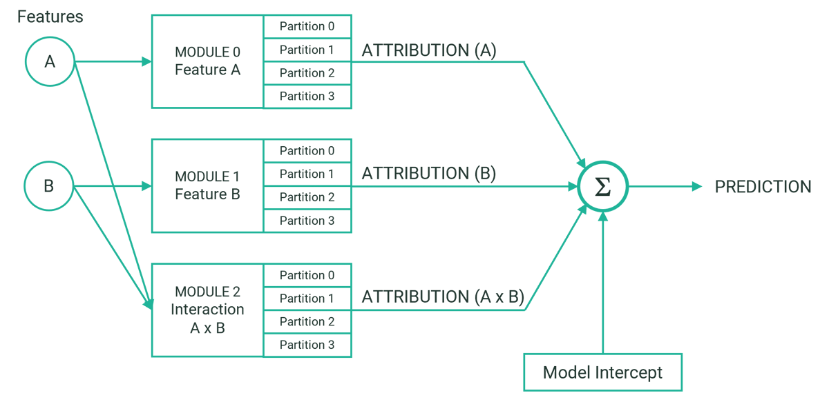
XNNs produce both a prediction and the raw explanation data behind it.

That explanation data is organised by the model’s structure:

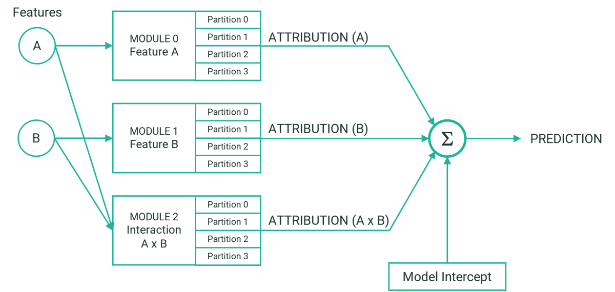
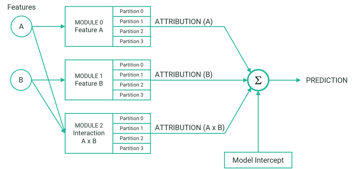
The sum of the module attributions, plus the model intercept, gives the prediction.

Module

An XNN is composed of modules.

Each module computes the attribution of one input feature or one feature interaction. A feature can contribute directly to the prediction, and it can also contribute through interactions with other features. In an XNN, each feature and feature interaction has its own module.

For example, a model may contain:

The attribution from each module describes how much that feature or interaction contributed to the prediction.

Partition

Each module contains one or more partitions.

A partition models the behaviour of a region of the input feature or interaction space. Partitions structure the knowledge discovered during induction: similar regions are grouped closer together, while dissimilar regions are kept further apart.

This arrangement forms a folder-like partition hierarchy, where related regions of behaviour are organised together.

The partition hierarchy allows the model to represent behaviour at different levels of detail. It also makes the model easier to inspect because related patterns are grouped together, helping people and machines process the information faster and see the broader structure of the model.

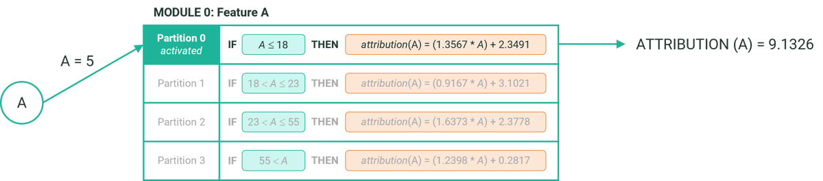
At inference time, exactly one partition is activated for each module.

Rule

Each partition has an associated rule.

A rule represents the knowledge learned for that partition as an IF-THEN statement:

IF <conditional_expression> THEN <then_expression>

The IF expression defines the conditions that activate the partition. The THEN expression defines the local neural model used to calculate the module attribution.

For a given data point, only one rule can trigger inside each module because rules within a module are non-overlapping.

For example, if a rule models the segment “females up to 23 years old”, its condition might be:

(0 < Age ≤ 23) AND (Gender = Female)

When that condition is true, the rule activates and the THEN expression calculates the attribution for the module.

Rules are useful because they make local model behaviour inspectable. They show which region activated, why it activated, and how the resulting contribution was calculated.

Bins

Bins define symbolic feature segments.

For numeric or sequential features, a bin usually represents a range of values. For categorical features, a bin can represent a category, or a group of categories.

Examples:

Bins are used to define the boundaries of partitions. A partition boundary may use one bin or a combination of bins, such as:

(0 < Age ≤ 18) AND (Gender = Female)

The bins and their combinations show how induction segmented the dataset into meaningful regions of behaviour.

Decompositions

Interaction modules can be broken down into feature-level components.

This process is called decomposition. A decomposition allocates the attribution of an interaction module across the features that participate in that interaction.

For example, a module for Age × Credit Score has one total attribution for the interaction. Decomposition makes it possible to assign part of that attribution to Age and part to Credit Score.

This is important for feature attribution: it allows interaction effects to be represented in terms of individual feature contributions while preserving fidelity.

Decomposition example

A partition in an Age × Credit Score module may calculate attribution as:

attribution(Age × Credit Score) = 0.07 + (0.018 * Age) + (0.0045 * Credit Score)

In this example, the interaction has two features and an intercept of 0.07.

For the Age decomposition:

age_terms = (0.018 * Age) + (0.0045 * Credit Score) / 2

all_terms = (0.018 * Age) + (0.0045 * Credit Score)

The decomposition equation for Age is:

attribution(Age) = age_terms + (age_terms / all_terms) * intercept + decomp_diff

Here, decomp_diff is the difference between the partition attribution and the sum of all decomposition attributions. It accounts for the intercept in the specific case where all module feature values are zero. In that case, decomp_diff is equal to the intercept.

For Age = 35 and Credit Score = 190, the result is:

The decomposition maintains fidelity:

attribution(Age) + attribution(Credit Score) = attribution(Age × Credit Score)

Intercept

The model intercept is the constant value added to the module attributions to produce the prediction.

It is also known as the bias term. Conceptually, it represents the model output when all feature values are zero.

Every prediction includes the intercept:

prediction = model_intercept + sum(module_attributions)

The intercept is useful when reconciling the prediction with the attribution values returned by views such as Results, Feature attribution, and Module attribution.